These are some tutorial /notes for Basic Electronics subject according to CSVTU syllabus.
Rapidshare link :
BE Unit 1
BE Unit 2
BE Unit 1 ppt
Megaupload Link :
BE Unit 1
BE Unit 2
BE unit 1 ppt
Complete All 5 units............
All 5 units
Happy Thinking Naturally..........
Showing posts with label Techie.... Show all posts
Showing posts with label Techie.... Show all posts
Friday, August 20, 2010

Sunday, August 02, 2009
Real men program in C
A very good article on C. A quite good comparative study of various famous programming languages with C. This is an article from "Embedded.com" so the article is based around embedded systems. Here is this Real men program in C.
Hope you will enjoy it.
Hope you will enjoy it.
Wednesday, July 22, 2009
Exploring Intel processors for SIMD support
As we already know that there are various way to speed up the processes or applications by parallel operations like Single Instruction Multiple Data(SIMD), multithreading, pipelining, cache management etc. Here I tried to manage a list of specifying which Intel SIMD capability we can use as per processor specific. Although you can check this by using CPU-Z or playing with cpu_detect() function to read cpu-id.
MMX: Truly saying as in 2009, all current processors support MMX. It has 8 registers MM0-MM7 of 64 bit width. Just to maintain uniformity of blog, MMX support came with Intel® Pentium-MMX and from Pentium2 onwards every processors support it.
SSE: It was another big move in SIMD by having another 128 bit registers by Intel. It is good choice for Intel® Pentium3 and Intel® Pentium3m version.
SSE2:
Intel® Xeon®
Intel® Pentium4 (Willamette),
Intel® Pentium4m,
Intel® Pentium M,
Intel NetBurst-based CPUs (Pentium 4, Xeon, Celeron, Celeron D, Celeron M)
Intel Core-based CPUs (Core Duo, Core Solo)
Intel Core 2-based CPUs (Core 2 Duo, Core 2 Quad)
Intel Atom
SSE3:
Dual-Core Intel® Xeon® 70XX, 71XX, 50XX Series
Dual-Core Intel® Xeon® processor (ULV and LV) 1.66, 2.0, 2.16
Dual-Core Intel® Xeon® 2.8
Intel® Xeon® processors with SSE3 instruction set support
Intel® Core™ Duo
Intel® Core™ Solo
Intel® Pentium® dual-core processor T21XX, T20XX series
Intel® Pentium® processor Extreme Edition (but NOT Pentium 4 Extreme Edition)
Intel® Pentium® D
Intel® Pentium® 4 processors with SSE3 instruction set support (Since Prescott Versions)
Celeron 420, 430 and 440 and Celeron D
Intel Core 2 Quad edition
Atom
SSSE3:
Quad-Core Intel® Xeon® 73XX, 53XX, 32XX series
Dual-Core Intel® Xeon® 72XX, 53XX, 51XX, 30XX series
In tel® Core™ 2 Extreme 7XXX, 6XXX series
Intel® Core™ 2 Quad 6XXX series
Intel® Core™ 2 Duo 7XXX (except E7200), 6XXX, 5XXX, 4XXX series
Intel® Core™ 2 Solo 2XXX series
Intel® Pentium® dual-core processor E2XXX, T23XX series
Celeron 4xx Sequence Conroe-L
Celeron Dual Core E1200
Celeron M 500 series
Atom
SSE4.1:
Intel® Xeon® 74XX series
Quad-Core Intel® Xeon 54XX, 33XX series
Dual-Core Intel® Xeon 52XX, 31XX series
Intel® Core™ 2 Extreme 9XXX series
Intel® Core™ 2 Quad 9XXX series
Intel® Core™ 2 Duo 8XXX series
Intel® Core™ 2 Duo E7200 (Penryn )
SSE4.2:
Intel® Core™ i7 Processors (Nehalem)
Intel® Xeon® 55XX series
Now play with SIMD with different processors options available.
MMX: Truly saying as in 2009, all current processors support MMX. It has 8 registers MM0-MM7 of 64 bit width. Just to maintain uniformity of blog, MMX support came with Intel® Pentium-MMX and from Pentium2 onwards every processors support it.
SSE: It was another big move in SIMD by having another 128 bit registers by Intel. It is good choice for Intel® Pentium3 and Intel® Pentium3m version.
SSE2:
Intel® Xeon®
Intel® Pentium4 (Willamette),
Intel® Pentium4m,
Intel® Pentium M,
Intel NetBurst-based CPUs (Pentium 4, Xeon, Celeron, Celeron D, Celeron M)
Intel Core-based CPUs (Core Duo, Core Solo)
Intel Core 2-based CPUs (Core 2 Duo, Core 2 Quad)
Intel Atom
SSE3:
Dual-Core Intel® Xeon® 70XX, 71XX, 50XX Series
Dual-Core Intel® Xeon® processor (ULV and LV) 1.66, 2.0, 2.16
Dual-Core Intel® Xeon® 2.8
Intel® Xeon® processors with SSE3 instruction set support
Intel® Core™ Duo
Intel® Core™ Solo
Intel® Pentium® dual-core processor T21XX, T20XX series
Intel® Pentium® processor Extreme Edition (but NOT Pentium 4 Extreme Edition)
Intel® Pentium® D
Intel® Pentium® 4 processors with SSE3 instruction set support (Since Prescott Versions)
Celeron 420, 430 and 440 and Celeron D
Intel Core 2 Quad edition
Atom
SSSE3:
Quad-Core Intel® Xeon® 73XX, 53XX, 32XX series
Dual-Core Intel® Xeon® 72XX, 53XX, 51XX, 30XX series
In tel® Core™ 2 Extreme 7XXX, 6XXX series
Intel® Core™ 2 Quad 6XXX series
Intel® Core™ 2 Duo 7XXX (except E7200), 6XXX, 5XXX, 4XXX series
Intel® Core™ 2 Solo 2XXX series
Intel® Pentium® dual-core processor E2XXX, T23XX series
Celeron 4xx Sequence Conroe-L
Celeron Dual Core E1200
Celeron M 500 series
Atom
SSE4.1:
Intel® Xeon® 74XX series
Quad-Core Intel® Xeon 54XX, 33XX series
Dual-Core Intel® Xeon 52XX, 31XX series
Intel® Core™ 2 Extreme 9XXX series
Intel® Core™ 2 Quad 9XXX series
Intel® Core™ 2 Duo 8XXX series
Intel® Core™ 2 Duo E7200 (Penryn )
SSE4.2:
Intel® Core™ i7 Processors (Nehalem)
Intel® Xeon® 55XX series
Now play with SIMD with different processors options available.
Thursday, July 02, 2009
How to make DLL and DLL Application in Visual Studio
Dynamic Linking Library (DLL) has the following advantages:
1) Saves memory and reduces swapping. Many processes can use a single DLL simultaneously, sharing a single copy of the DLL in memory. In contrast, Windows must load a copy of the library code into memory for each application that is built with a static link library.
2) Saves disk space. Many applications can share a single copy of the DLL on disk. In contrast, each application built with a static link library has the library code linked into its executable image as a separate copy.
3) Upgrades to the DLL are easier. When the functions in a DLL change, the applications that use them do not need to be recompiled or relinked as long as the function arguments and return values do not change. In contrast, statically linked object code requires that the application be relinked when the functions change.
4) Provides after-market support. For example, a display driver DLL can be modified to support a display that was not available when the application was shipped.
5) Supports multi-language programs. Programs written in different programming languages can call the same DLL function as long as the programs follow the function's calling convention. The programs and the DLL function must be compatible in the following ways: the order in which the function expects its arguments to be pushed onto the stack, whether the function or the application is responsible for cleaning up the stack, and whether any arguments are passed in registers.
6)Eases the creation of international versions. By placing resources in a DLL, it is much easier to create international versions of an application. You can place the strings for each language version of your application in a separate resource DLL and have the different language versions load the appropriate resources.
A potential disadvantage to using DLLs is that the application is not self-contained; it depends on the existence of a separate DLL module.
With the use of dll's one application can use or perform multiple functionality by using multiple dll's. And another advantage is you dont have to give full code, just give applicxation .exe along with Library .dll and that 's enough to run the code.
To make an application by using dll, we need two different projects. One project will be Libarary for which we will make .dll and another will be appplication i.e. .exe file.
Ok let's start with Library project. Followings will be the steps:
1) Open visual studio and go to New Project. Choose "Win32 console project"
2) In application setting, choose DLL.
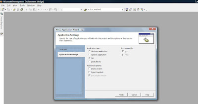
3) You will get 3 files in your project.
a) Dll_main.cpp b) stdafx.cpp and c) stdafx.h
you will also get some code already avaiable to those files. Just Keep it, those are required for compiler as an entry point to .dll
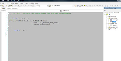
4) Now write your code or functions as usual only without main(). As main() will be in application project. Only thing is that the functions which will be avaialbe to applications, should to be exported. To export the function , you have to add "__declspec(dllexport)" before return type of function. I use define something like this
#define DLL_EXPORT __declspec(dllexport)
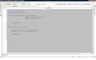 and header file will be
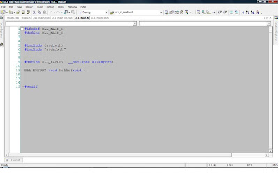
5) Other functions will be normal. no extra prefix. Just like I am using 'InsideHello()'in my DLL main.
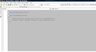
6) Now go to project porpoety page, and to C/C++ section , and set "Not Using Precompiled Headers"
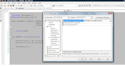
7) Now build the project, after successful build you will get ProjectName.lib and ProjectName.dll, so as for my case DLL_Lib.lib and DLL_Lib.dll. So you got your required .dll and .lib which we need for building application.
Now open new project for application. All settings will be normal as we do for usual .exe application.
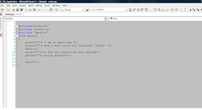
and exported function of DLL_lib should be imported here by adding "__declspec(dllimport) " before return type of those function.
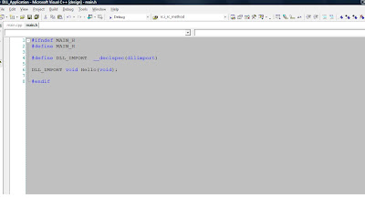
And now you have to add dependencies, for that go to property page and linker section and add as "input" the .llib file, for my case DLL_Lib.lib (which contain declarion of functions.)
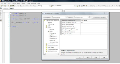
And copy the .lib and .dll from the Library project in the folder where .sln is present of application project. That's it, now build the project, if build successful i.e. your application has taken .lib and .dll and can be used. So now for test, keep .exe application and .dll of lib anywhere, it will run properly.
Now if you want handle totally different functionality, by only one application, make diffrerent .dll's and use there functions in your application. just like i was testing, two .dll in one exe.both written separately, but later thought to use in one application.
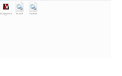 Enjoy .dll applications now!!!!
1) Saves memory and reduces swapping. Many processes can use a single DLL simultaneously, sharing a single copy of the DLL in memory. In contrast, Windows must load a copy of the library code into memory for each application that is built with a static link library.
2) Saves disk space. Many applications can share a single copy of the DLL on disk. In contrast, each application built with a static link library has the library code linked into its executable image as a separate copy.
3) Upgrades to the DLL are easier. When the functions in a DLL change, the applications that use them do not need to be recompiled or relinked as long as the function arguments and return values do not change. In contrast, statically linked object code requires that the application be relinked when the functions change.
4) Provides after-market support. For example, a display driver DLL can be modified to support a display that was not available when the application was shipped.
5) Supports multi-language programs. Programs written in different programming languages can call the same DLL function as long as the programs follow the function's calling convention. The programs and the DLL function must be compatible in the following ways: the order in which the function expects its arguments to be pushed onto the stack, whether the function or the application is responsible for cleaning up the stack, and whether any arguments are passed in registers.
6)Eases the creation of international versions. By placing resources in a DLL, it is much easier to create international versions of an application. You can place the strings for each language version of your application in a separate resource DLL and have the different language versions load the appropriate resources.
A potential disadvantage to using DLLs is that the application is not self-contained; it depends on the existence of a separate DLL module.
With the use of dll's one application can use or perform multiple functionality by using multiple dll's. And another advantage is you dont have to give full code, just give applicxation .exe along with Library .dll and that 's enough to run the code.
To make an application by using dll, we need two different projects. One project will be Libarary for which we will make .dll and another will be appplication i.e. .exe file.
Ok let's start with Library project. Followings will be the steps:
1) Open visual studio and go to New Project. Choose "Win32 console project"
2) In application setting, choose DLL.

3) You will get 3 files in your project.
a) Dll_main.cpp b) stdafx.cpp and c) stdafx.h
you will also get some code already avaiable to those files. Just Keep it, those are required for compiler as an entry point to .dll

4) Now write your code or functions as usual only without main(). As main() will be in application project. Only thing is that the functions which will be avaialbe to applications, should to be exported. To export the function , you have to add "__declspec(dllexport)" before return type of function. I use define something like this
#define DLL_EXPORT __declspec(dllexport)
 and header file will be
5) Other functions will be normal. no extra prefix. Just like I am using 'InsideHello()'in my DLL main.

6) Now go to project porpoety page, and to C/C++ section , and set "Not Using Precompiled Headers"

7) Now build the project, after successful build you will get ProjectName.lib and ProjectName.dll, so as for my case DLL_Lib.lib and DLL_Lib.dll. So you got your required .dll and .lib which we need for building application.
Now open new project for application. All settings will be normal as we do for usual .exe application.

and exported function of DLL_lib should be imported here by adding "__declspec(dllimport) " before return type of those function.

And now you have to add dependencies, for that go to property page and linker section and add as "input" the .llib file, for my case DLL_Lib.lib (which contain declarion of functions.)

And copy the .lib and .dll from the Library project in the folder where .sln is present of application project. That's it, now build the project, if build successful i.e. your application has taken .lib and .dll and can be used. So now for test, keep .exe application and .dll of lib anywhere, it will run properly.
Now if you want handle totally different functionality, by only one application, make diffrerent .dll's and use there functions in your application. just like i was testing, two .dll in one exe.both written separately, but later thought to use in one application.
 Enjoy .dll applications now!!!!
Sunday, June 14, 2009
Google Wave: A new way of Browsing
How many times you felt like you need multiple browsers to open various communication formats like 'email', 'chat', 'docs', 'blogs', 'youtube' etc. etc. while discussing with only one friend. You also might have thought Why I cant share all my docs in one place , so that everybody like my friend or team can see it and can discuss everything here at one browser in real time. Many times it happens to me like my friend tell me check this page or video or doc, he gives me link, I copy the link and open another browser and check it, sometimes link work and sometimes doesn't. Even if it works, he has to wait for me to finish reading it and come back to start discussion. Now while discussion we need to switch between the doc window and chat window multiple times, really frustrating........
Thanks to google that after few more months wait, this problem is going to resolved like forever. Google has launched the new open source product called 'Google Wave' . "Google Wave" is equal parts conversation and document, where people can communicate and work together with richly formatted text, photos, videos, maps, and more.

In a simple form Google Wave is nothing but a combination of gmail, gtalk, google docs, blogger, google map, video etc etc. truly saying a combo of all, and even I can say more than that. As it is open source product, so it is also a platform with a rich set of open APIs (google wave API )that allow developers to embed waves in other web services and to build extensions that work inside waves.

Google Wave has been designed by the founders of Where 2 Tech, a start-up acquired by Google to create a cutting-edge mapping service, which later became Google Maps. According to Lars Rasmussen "In Google Wave you create a wave and add people to it. Everyone on your wave can use richly formatted text, photos, gadgets, and even feeds from other sources on the web. They can insert a reply or edit the wave directly. It's concurrent rich-text editing, where you see on your screen nearly instantly what your fellow collaborators are typing in your wave. That means Google Wave is just as well suited for quick messages as for persistent content -- it allows for both collaboration and communication. You can also use "playback" to rewind the wave to see how it evolved."

It includes a rich text editor and other functions like desktop drag-and-drop (which, for example, lets you drag a set of photos right into a wave).

You can add person, chat with them, share videos, discuss about location all in real time.

As "Wave" has google wave extension so it means there are a numbers of applications available that can be used and there will be mutiple users available for interaction like playing online games such as sudoku, scramble, chess etc.

One more interesting thing is you have google map available there, so ask your friends to join for party and give the location in "Wave" using google map, get their reply immediately. Something like this.

Believe me there are a lot many other stuffs too, when you will use it , you will just say "Awesome". To know more about it, check my "Important links" sections at the last of this post.
PS: Google Wave is currently available in a developer preview as the APIs and product continue to evolve. Accounts on the developer sandbox will be given out to people intending to build with the Google Wave APIs prior to the public release.
So if you are developer and want to contribute, go get your "Wave" or wait for release mode for a few months. if you'd like to be notified when we launch Google Wave as a public product, you can sign up at here.
Important links:
1) Google Wave
2) Google Wave Developer Blog
3) Intoducing the Google Wave APIs
4) Google Wave Code Blog
5) About Google Wave
6) Google Wave: A Complete Guide
7) Google Wave Extensions: An Inside Look
Thanks to google that after few more months wait, this problem is going to resolved like forever. Google has launched the new open source product called 'Google Wave' . "Google Wave" is equal parts conversation and document, where people can communicate and work together with richly formatted text, photos, videos, maps, and more.

In a simple form Google Wave is nothing but a combination of gmail, gtalk, google docs, blogger, google map, video etc etc. truly saying a combo of all, and even I can say more than that. As it is open source product, so it is also a platform with a rich set of open APIs (google wave API )that allow developers to embed waves in other web services and to build extensions that work inside waves.

Google Wave has been designed by the founders of Where 2 Tech, a start-up acquired by Google to create a cutting-edge mapping service, which later became Google Maps. According to Lars Rasmussen "In Google Wave you create a wave and add people to it. Everyone on your wave can use richly formatted text, photos, gadgets, and even feeds from other sources on the web. They can insert a reply or edit the wave directly. It's concurrent rich-text editing, where you see on your screen nearly instantly what your fellow collaborators are typing in your wave. That means Google Wave is just as well suited for quick messages as for persistent content -- it allows for both collaboration and communication. You can also use "playback" to rewind the wave to see how it evolved."

It includes a rich text editor and other functions like desktop drag-and-drop (which, for example, lets you drag a set of photos right into a wave).

You can add person, chat with them, share videos, discuss about location all in real time.

As "Wave" has google wave extension so it means there are a numbers of applications available that can be used and there will be mutiple users available for interaction like playing online games such as sudoku, scramble, chess etc.

One more interesting thing is you have google map available there, so ask your friends to join for party and give the location in "Wave" using google map, get their reply immediately. Something like this.

Believe me there are a lot many other stuffs too, when you will use it , you will just say "Awesome". To know more about it, check my "Important links" sections at the last of this post.
PS: Google Wave is currently available in a developer preview as the APIs and product continue to evolve. Accounts on the developer sandbox will be given out to people intending to build with the Google Wave APIs prior to the public release.
So if you are developer and want to contribute, go get your "Wave" or wait for release mode for a few months. if you'd like to be notified when we launch Google Wave as a public product, you can sign up at here.
Important links:
1) Google Wave
2) Google Wave Developer Blog
3) Intoducing the Google Wave APIs
4) Google Wave Code Blog
5) About Google Wave
6) Google Wave: A Complete Guide
7) Google Wave Extensions: An Inside Look
Thursday, June 11, 2009
How to include YASM in Visual Studio 2005
Playing with SIMD or assembly is very enjoyable thing, you will love coding here. But believe me actual fun starts when you use on NASM or YASM to write assembly rather than working with IA32 inline (__Asm{...}) assembly development coding method. YASM has included some more features than NASM but the real issue with NASM is the limited debugging formats. Debugger available in NASM are for 'stabs'and 'dwarf2' only. If you work on visual studio than NASM no use. NASM will assemble the code but you can not debug the code. So the best choice is YASM.
YASM can be downloaded from here. YASM supports various output format and supports debug formats 'stabs', 'dwarf2' and 'CodeView (cv)' check this. So it can be included in Visual Studio 2005 for assembly/SIMD code development.
So today we will discuss about how to include YASM assembler in visual studio 2005 project. We will go step by step for better understanding. So here we goes:
1) Download the latest YASM.exe, if donwloaded Yasm executable binary is not named as yasm.exe; we have to rename it yasm.exe.
2) Go to directory "Program Files\Microsoft Visual Studio 8\VC\bin" where all VC related binaries are kept already and put yasm.exe into it.
3) Now you need file named as 'yasm.rules'. To get this, download latest source code of YASM. Actually you can build yasm.exe with this source project also, but I am not concern with that today . Now locate folder "\Mkfiles\vc8" in yasm folder, you will find 'yasm.rules' file there.
4) To use custom build tool of visual studio 2005, copy 'yasm.rules' file to "Program Files\Microsoft Visual Studio 8\VC\VCProjectDefaults".
5) Now simply write your assembly in a file added to your project with file extension '.asm'
6) To assemble a file with Yasm, select the Property Page for the file and the select Yasm Assembler in the Tool dialog entry. Then add following line to 'Misc' section in 'command line' menu of property page :-
Debug mode : yasm -f win32 -g cv8 -o "$(IntDir)\$(InputName)".obj "$(InputPath)"
Release Mode : yasm -f win32 -o "$(IntDir)\$(InputName)".obj "$(InputPath)"
Press Apply and you are done. Now enjoy SIMD/assembly with YASM in Visual studio 2005.
I hope, you will find this article useful.
Useful links:
1) YASM in Wiki
2) YASM Home page
3) Latest version for download
4) YASM Documentation
5) YASM in VS 2005
YASM can be downloaded from here. YASM supports various output format and supports debug formats 'stabs', 'dwarf2' and 'CodeView (cv)' check this. So it can be included in Visual Studio 2005 for assembly/SIMD code development.
So today we will discuss about how to include YASM assembler in visual studio 2005 project. We will go step by step for better understanding. So here we goes:
1) Download the latest YASM.exe, if donwloaded Yasm executable binary is not named as yasm.exe; we have to rename it yasm.exe.
2) Go to directory "Program Files\Microsoft Visual Studio 8\VC\bin" where all VC related binaries are kept already and put yasm.exe into it.
3) Now you need file named as 'yasm.rules'. To get this, download latest source code of YASM. Actually you can build yasm.exe with this source project also, but I am not concern with that today . Now locate folder "\Mkfiles\vc8" in yasm folder, you will find 'yasm.rules' file there.
4) To use custom build tool of visual studio 2005, copy 'yasm.rules' file to "Program Files\Microsoft Visual Studio 8\VC\VCProjectDefaults".
5) Now simply write your assembly in a file added to your project with file extension '.asm'
6) To assemble a file with Yasm, select the Property Page for the file and the select Yasm Assembler in the Tool dialog entry. Then add following line to 'Misc' section in 'command line' menu of property page :-
Debug mode : yasm -f win32 -g cv8 -o "$(IntDir)\$(InputName)".obj "$(InputPath)"
Release Mode : yasm -f win32 -o "$(IntDir)\$(InputName)".obj "$(InputPath)"
Press Apply and you are done. Now enjoy SIMD/assembly with YASM in Visual studio 2005.
I hope, you will find this article useful.
Useful links:
1) YASM in Wiki
2) YASM Home page
3) Latest version for download
4) YASM Documentation
5) YASM in VS 2005
Sunday, June 07, 2009
Clip Signed Data To Arbitrary Unsigned Range in SIMD/Assembly
This post is again dedicated to Video domain. But I certainly can say there are various other applications too where we can use it.
Clipping is very simple algorithm as it name indicates, we clip our data to certain range. There will be High value and Low value. If data value is less than Low value, assign data to Low and if data value goes upper than High value assign data to High. something like this:
Clip(Data,Low,High) = if Data is less than Low then data = Low, else if Data is greater than High then data= High , else data = Data ------------(1)
In video domain, after IDCT operation we get signed data for pixel, which should be technically unsigned data type. Here we do clip operation for pixel data, and limit the data between unsigned data type range, and in normal situation pixel bit depth is 8 (i.e unsigned char). So equ. (1) becomes :
Clip(Data,0,255) =if Data is less than 0 then data = 0, else if Data is greater than 255 data= 255, else data = Data ------------------------(2)
But pixel bit-depth is not limited to 8. As I mentioned in my previous post "H264:How to do conversion from 8 bits to 14 bits bit depth support" under the label "Video", H.264 support till 14 bit bit-depth, when you don't want to compromise with quality, go for higher bit -depth. And here pixel data type will be 'unsigned short'. Now we have to modify the 'Clip' function for higher bit-depth. And this time it is not fixed to 8 and not even 14, rather it can vary from 8 to 14 depends upon the YUV input bit-depth for encoder and luma or chroma bit-depth information (bit_depth_luma_minus8 and bit_depth_chroma_minus8) from input H.264 coded video input for decoder. So lets do this clipping in generic form. And remember Low value will be 0 always only High value will change. So equ (2) modified as :
High = (1^Pixel_Bit_Depth)-1
Clip(Data, 0, High) = if Data is less than 0 then data = 0, else if Data is greater than High then data= High , else data = Data ------------------------(3)
There are other optimized ways too for equ.(3), but that's not my concern as of today. so moving ahead for SIMD/assembly (MMX/SSE/SSE2). Now how to achieve the same operation in assembly. Actually if bit-depth is 8 then there is a single instruction available in SIMD as :
packuswb Rx0, Rx0 ;Considered data is in Rx0 (mm/xmm) SIMD register (if pixel type is unsigned char)
or if Rx1 is '0' then
paddusb Rx0, Rx1
if you want to saturate for unsigned short then we have
paddusw Rx0, Rx1
But that is not our case, so we have to go by other way. As we have data type 'unsigned short ' and Max value will be (1^Pixel_Bit_Depth)-1 , So here we goes :
unsigned short High = (1^Pixel_Bit_Depth)-1
unsigned short Range = 0x8000;
unsigned short Low = 0x7FFF - High;
unsigned short MaxHigh = 0xFFFF - High;
movdqu Rx1, Range
movdqu Rx2, Low
movdqu Rx3, MaxHigh
paddw Rx0, Rx1
paddusw Rx0, Rx2 ;Add unsigned saturation with Low
psubusw Rx0, Rx3 ;Subtract unsigned saturation with MaxHigh
(Note above code instructions are for SSE2 but applied for MMX too, also I tried to wrote for one pixel data, to use SIMD advantage properly some data shuffling is required, here my intention was to give idea, not the complete code for cut n paste.)
Enjoy!!!!
Clipping is very simple algorithm as it name indicates, we clip our data to certain range. There will be High value and Low value. If data value is less than Low value, assign data to Low and if data value goes upper than High value assign data to High. something like this:
Clip(Data,Low,High) = if Data is less than Low then data = Low, else if Data is greater than High then data= High , else data = Data ------------(1)
In video domain, after IDCT operation we get signed data for pixel, which should be technically unsigned data type. Here we do clip operation for pixel data, and limit the data between unsigned data type range, and in normal situation pixel bit depth is 8 (i.e unsigned char). So equ. (1) becomes :
Clip(Data,0,255) =if Data is less than 0 then data = 0, else if Data is greater than 255 data= 255, else data = Data ------------------------(2)
But pixel bit-depth is not limited to 8. As I mentioned in my previous post "H264:How to do conversion from 8 bits to 14 bits bit depth support" under the label "Video", H.264 support till 14 bit bit-depth, when you don't want to compromise with quality, go for higher bit -depth. And here pixel data type will be 'unsigned short'. Now we have to modify the 'Clip' function for higher bit-depth. And this time it is not fixed to 8 and not even 14, rather it can vary from 8 to 14 depends upon the YUV input bit-depth for encoder and luma or chroma bit-depth information (bit_depth_luma_minus8 and bit_depth_chroma_minus8) from input H.264 coded video input for decoder. So lets do this clipping in generic form. And remember Low value will be 0 always only High value will change. So equ (2) modified as :
High = (1^Pixel_Bit_Depth)-1
Clip(Data, 0, High) = if Data is less than 0 then data = 0, else if Data is greater than High then data= High , else data = Data ------------------------(3)
There are other optimized ways too for equ.(3), but that's not my concern as of today. so moving ahead for SIMD/assembly (MMX/SSE/SSE2). Now how to achieve the same operation in assembly. Actually if bit-depth is 8 then there is a single instruction available in SIMD as :
packuswb Rx0, Rx0 ;Considered data is in Rx0 (mm/xmm) SIMD register (if pixel type is unsigned char)
or if Rx1 is '0' then
paddusb Rx0, Rx1
if you want to saturate for unsigned short then we have
paddusw Rx0, Rx1
But that is not our case, so we have to go by other way. As we have data type 'unsigned short ' and Max value will be (1^Pixel_Bit_Depth)-1 , So here we goes :
unsigned short High = (1^Pixel_Bit_Depth)-1
unsigned short Range = 0x8000;
unsigned short Low = 0x7FFF - High;
unsigned short MaxHigh = 0xFFFF - High;
movdqu Rx1, Range
movdqu Rx2, Low
movdqu Rx3, MaxHigh
paddw Rx0, Rx1
paddusw Rx0, Rx2 ;Add unsigned saturation with Low
psubusw Rx0, Rx3 ;Subtract unsigned saturation with MaxHigh
(Note above code instructions are for SSE2 but applied for MMX too, also I tried to wrote for one pixel data, to use SIMD advantage properly some data shuffling is required, here my intention was to give idea, not the complete code for cut n paste.)
Enjoy!!!!
Thursday, May 21, 2009
SSE2 Vs SSSE3
As you already know that I am a bit busy with learning intel SIMD like mmx, sse2 , ssse3 etc stuff. I am enjoying SIMD and playing with all these MMX, SSE versions.While working with SSSE3 after sse2 or sse3, I thought what is the advantage of SSSE3 over SSE2? Some people even ask me why there is not a dramatic change in performance after adding SSSE3. I knew the answer but thought to do some more R&D on it.
And here is my view....
I will start with some brief intro of SSE versions and also as I am in video field I will talk about integer operations only that will be my primary concern as of now.
SSE2 instructions are an extension of the SIMD introduced with the MMX technology and the SSE extensions.The key benefits of SSE2 are that both MMX ans SSE2 instructions can work on 8 XMM (128-bit, XMM0- XMM7) register along with the MMX registers (mm0-mm7), and that SSE instructions now support 64-bit floating-point values. So there was huge change between MMX and SSE2(or SSE). Now because of XMM registers instead of playing with 8 bytes, we can play 16 bytes simultaneously. So improving the performance just by double from the MMX assembly or 16 times from the C code. There are some instructions we are missing in MMX assembly which are present in SSE2 like paddsb/w, movapd,movupd, pshufw/d ,pavgb/w etc, which are very much helpful here in video compression.
While SSSE3 (Supplemental Streaming SIMD Extension 3) is an extension of SSE3 or I should say revision of SSE3. In SSE3(13 new instructions) the most notable change is the capability to work horizontally in a register, as opposed to the more or less strictly vertical operation of all previous SSE instructions. There are instructions to add and subtract the multiple values stored within a single register have been added. But note those are not for Integer operations only floating point, that's why I am talking about SSSE3.
SSSE3 contains 16 new discrete instructions over SSE3. Each can act on 64-bit MMX or 128-bit XMM registers. Therefore, Intel's manuals has 32 new instructions.The instructions are PSIGNB/W/D, PABSB/W/D, PALIGNR, PSHUFB, PMULHRSW, PMADDUBSW, PHSUBW/D, PHSUBSW, PHADDW/D and PHADDSW.So if you these, the processing block or registers are same as SSE2, no new registers.
By using SSSE3 the only advantage in video compression side integer operations is horizontally processing. So by SSSE3 we can add/subtract the data within the registers instead of adding or subtracting with other registers. So I feel SSSE3 only removes some overheads and save some cycles by using horizontal operations if your video code is having that kind of module like SAD, SSD and all, but there are be many places where transition from MMX to SSE2 gives huge improvement in performance but transition from SSE2 to SSSE3 may not give you even noticeable change. Even there will be lots of functions where SSSE3 will not be required over SSE2 in code. As to work vertically (between two registers) we sometimes do some data manipulations by padding 0's or by shuffling data between registers, and then process the data like addition/multiplication etc., those shuffling or padding are overheads that can be avoided here in SSSE3.
I guess we should not think that each next generation of SIMD will just magically double the performance of the code same like MMX to SSE/SSE2. Function module (like DCT, SAD etc.) and data fetching to those functions matters a lot to decide which SIMD we should use .... SSE2 or SSSE3 for better performance. So before converting any new code from SSE2 to SSSE3, just stop for a moment, have a close look on the module and then choose SSE2 Vs SSSE3.
Enjoy SIMD optimization.
And here is my view....
I will start with some brief intro of SSE versions and also as I am in video field I will talk about integer operations only that will be my primary concern as of now.
SSE2 instructions are an extension of the SIMD introduced with the MMX technology and the SSE extensions.The key benefits of SSE2 are that both MMX ans SSE2 instructions can work on 8 XMM (128-bit, XMM0- XMM7) register along with the MMX registers (mm0-mm7), and that SSE instructions now support 64-bit floating-point values. So there was huge change between MMX and SSE2(or SSE). Now because of XMM registers instead of playing with 8 bytes, we can play 16 bytes simultaneously. So improving the performance just by double from the MMX assembly or 16 times from the C code. There are some instructions we are missing in MMX assembly which are present in SSE2 like paddsb/w, movapd,movupd, pshufw/d ,pavgb/w etc, which are very much helpful here in video compression.
While SSSE3 (Supplemental Streaming SIMD Extension 3) is an extension of SSE3 or I should say revision of SSE3. In SSE3(13 new instructions) the most notable change is the capability to work horizontally in a register, as opposed to the more or less strictly vertical operation of all previous SSE instructions. There are instructions to add and subtract the multiple values stored within a single register have been added. But note those are not for Integer operations only floating point, that's why I am talking about SSSE3.
SSSE3 contains 16 new discrete instructions over SSE3. Each can act on 64-bit MMX or 128-bit XMM registers. Therefore, Intel's manuals has 32 new instructions.The instructions are PSIGNB/W/D, PABSB/W/D, PALIGNR, PSHUFB, PMULHRSW, PMADDUBSW, PHSUBW/D, PHSUBSW, PHADDW/D and PHADDSW.So if you these, the processing block or registers are same as SSE2, no new registers.
By using SSSE3 the only advantage in video compression side integer operations is horizontally processing. So by SSSE3 we can add/subtract the data within the registers instead of adding or subtracting with other registers. So I feel SSSE3 only removes some overheads and save some cycles by using horizontal operations if your video code is having that kind of module like SAD, SSD and all, but there are be many places where transition from MMX to SSE2 gives huge improvement in performance but transition from SSE2 to SSSE3 may not give you even noticeable change. Even there will be lots of functions where SSSE3 will not be required over SSE2 in code. As to work vertically (between two registers) we sometimes do some data manipulations by padding 0's or by shuffling data between registers, and then process the data like addition/multiplication etc., those shuffling or padding are overheads that can be avoided here in SSSE3.
I guess we should not think that each next generation of SIMD will just magically double the performance of the code same like MMX to SSE/SSE2. Function module (like DCT, SAD etc.) and data fetching to those functions matters a lot to decide which SIMD we should use .... SSE2 or SSSE3 for better performance. So before converting any new code from SSE2 to SSSE3, just stop for a moment, have a close look on the module and then choose SSE2 Vs SSSE3.
Enjoy SIMD optimization.
Friday, April 17, 2009
NGVC (H.265) Is On The way
While the whole multimedia world trying very hard to become mature in H.264, the bestcompression video standard till today, the new baby is in under development phase and named as 'The Next Generation Video Coding' (NCVG). In 2005 it was started by VCEG as consideration to 'H.264+'. Then after study it changed to H.265 a brand new standard instead of an extension of H.264 as a long-term video coding standard. And now latest VCEG meeting it has came up as 'NGVC' project (next-generation video coding) with backward compatibility. It is expected to be finalized in 2009-2010.
The goal of this standardization will be as follows:
1. Coding efficiency:
* NGVC should be capable of providing a bit rate reduction of 50% at the same subjective quality
2. Complexity:
* NGVC should be capable of operating with a complexity ranging from 50% to 3 times H.264/MPEG-4 AVC High Profile.
* When operated at a complexity of 50% compared to H.264/MPEG-4 AVC High Profile, NGVC should provide a 25% bit rate savings compared to H.264/MPEG-4 AVC High Profile at equivalent subjective quality.
3. Applications:
* Low-delay interactive video communications
* Surveillance
* Streaming
* Broadcast
* Digital cinema and large-screen digital imagery
* Mobile video entertainment
* Storage-based video application (camcorders, camera phones, computer files, disc media, download-and-play, etc)
KTA (key technical area) is developed as the software platform, which uses JM11 as the baseline and continuously integrates promising coding tools. The tools adopted in KTA are listed as below:
* 2-D non-separable adaptive interpolation filter (AIF) [AD08]
* separable AIF [C-0219-E]
* directional AIF [AG21]
* motion compensation with 1/8-pel motion vectors [AD09]
* adaptive prediction error coding (APEC) in spatial and frequency domain [AD07]
* adaptive quantization matrix selection (AQMS) [AD06]
* competition-based scheme for motion vector selection and coding [AC06]
* mode-dependent transform customization for intra coding [AG11]
All these techniques improve the coding performance by multi-pass encoding.
The latest published KTA software is JM11.0KTA2.3 (download here ). Some new technologies have been adopted by KTA software since July 2008. Those KTA coding tools involve the following areas:
1. Architecture
Internal Bit Depth Increasing
Extended Block Size (or called Super-MacroBlock) (C123)
2. Transformation and Quantization
Mode-Dependent Directional Transform
Very Large Block Transform
Adaptive Prediction Error Coding
Improved Adaptive Quantization Matrix Selection
Rate-Distortion-Optimization Quantization (RDO-Q)
Adaptive QP
3. Entropy Coding
Parallel Entropy Coding
4. Adaptive Loop Filter
Block/Quadtree-based Adaptive Loop Filter (C181)
5. Motion Coding
Motion Vector Prediction Competition
One-eighth-sample Motion Vector Resolution
6. Inter-Prediction
Adaptive Interpolation Filters
Separable Adaptive Interpolation Filters
Directional Adaptive Interpolation Filters
Enhanced Adaptive Interpolation Filter
Enhanced Directional Adaptive Interpolation Filter
Fixed Directional Interpolation Filters
Special Filter Positions
High Precision Filters
Switched Interpolation Filters with Offsets
These are some related helpful links:
1) ITU-T SG16’s homepage
2) The latest version of KTA is JM11.0KTA2.3 (Download here) and the latest test conditions are specified in [AH10].
3) H265.net forum instead use this H.265.net (modifying after a valuable comment...thanks for rectifying me)
So be ready to see new fun in video coding.
The goal of this standardization will be as follows:
1. Coding efficiency:
* NGVC should be capable of providing a bit rate reduction of 50% at the same subjective quality
2. Complexity:
* NGVC should be capable of operating with a complexity ranging from 50% to 3 times H.264/MPEG-4 AVC High Profile.
* When operated at a complexity of 50% compared to H.264/MPEG-4 AVC High Profile, NGVC should provide a 25% bit rate savings compared to H.264/MPEG-4 AVC High Profile at equivalent subjective quality.
3. Applications:
* Low-delay interactive video communications
* Surveillance
* Streaming
* Broadcast
* Digital cinema and large-screen digital imagery
* Mobile video entertainment
* Storage-based video application (camcorders, camera phones, computer files, disc media, download-and-play, etc)
KTA (key technical area) is developed as the software platform, which uses JM11 as the baseline and continuously integrates promising coding tools. The tools adopted in KTA are listed as below:
* 2-D non-separable adaptive interpolation filter (AIF) [AD08]
* separable AIF [C-0219-E]
* directional AIF [AG21]
* motion compensation with 1/8-pel motion vectors [AD09]
* adaptive prediction error coding (APEC) in spatial and frequency domain [AD07]
* adaptive quantization matrix selection (AQMS) [AD06]
* competition-based scheme for motion vector selection and coding [AC06]
* mode-dependent transform customization for intra coding [AG11]
All these techniques improve the coding performance by multi-pass encoding.
The latest published KTA software is JM11.0KTA2.3 (download here ). Some new technologies have been adopted by KTA software since July 2008. Those KTA coding tools involve the following areas:
1. Architecture
Internal Bit Depth Increasing
Extended Block Size (or called Super-MacroBlock) (C123)
2. Transformation and Quantization
Mode-Dependent Directional Transform
Very Large Block Transform
Adaptive Prediction Error Coding
Improved Adaptive Quantization Matrix Selection
Rate-Distortion-Optimization Quantization (RDO-Q)
Adaptive QP
3. Entropy Coding
Parallel Entropy Coding
4. Adaptive Loop Filter
Block/Quadtree-based Adaptive Loop Filter (C181)
5. Motion Coding
Motion Vector Prediction Competition
One-eighth-sample Motion Vector Resolution
6. Inter-Prediction
Adaptive Interpolation Filters
Separable Adaptive Interpolation Filters
Directional Adaptive Interpolation Filters
Enhanced Adaptive Interpolation Filter
Enhanced Directional Adaptive Interpolation Filter
Fixed Directional Interpolation Filters
Special Filter Positions
High Precision Filters
Switched Interpolation Filters with Offsets
These are some related helpful links:
1) ITU-T SG16’s homepage
2) The latest version of KTA is JM11.0KTA2.3 (Download here) and the latest test conditions are specified in [AH10].
3) H265.net forum instead use this H.265.net (modifying after a valuable comment...thanks for rectifying me)
So be ready to see new fun in video coding.
Sunday, April 05, 2009
March-April Update (MMX Techonoly/NASM/YASM)
I see that my planned tasks are completely frozen from last one month. Many things happened in last month which stopped my scheduled work. I had to go out of town for 15 Days, when I came back there was huge amount of work in my office. Not only huge, the overall whole work is new for me. So I am not at all getting anytime for my blog. Actually I do find a little bit time to write blog but I dont have time to do my planned technical KEP as per scheduled. But the good thing is as I told earlier I doing some new things in work, at least that is satisfactory and I am enjoying there.
Presently I am working on MMX technology. I am quite busy in writing MMX assemblies. Basically it is SIMD (single instruction multiple data) technology where we use 64 bit 8 MMX registers (MM0-MM7) to process data. So if we have data of 'char' type so we can process 8 data simlataneously.There are various instructions which Pack or unpack multiple data and operations for 1 Quand Word(64 bit), 2 Double Word(32 bit), 4 Word(16 bit) or 8 Byte(8 bit) data depends upon how we handle the data.It's quite interesting.
Now for MMX instruction assemblies I am also learning the IA32 assembler, NASM (Netwide Assembler) and also YASM. The IA32 architecture is good but not sufficient as it will support only Intel architecture ( 80x86 assembler) and writing code as inline __asm {...} without using MACRO, repeat (loop) feature is highly tedious job. NASM is an 80x86 assembler designed for portability and modularity. It supports a range of object file formats, including Linux and NetBSD/FreeBSD a.out ,ELF , COFF , Microsoft 16-bit OBJ and Win32 . It will also output plain binary files. Its syntax is designed to be simple and easy to understand, similar to Intel’s but less complex. It supports Pentium , P6 , MMX , 3DNow! , SSE and SSE2 opcodes, and has macro capability.
While Yasm is a (mostly) BSD-licensed assembler that is designed from the ground up to allow for multiple assembler syntaxes to be supported (e.g. NASM, GNU AS, etc.) in addition to multiple output object formats and multiple instruction sets. Its modular architecture allows additional object formats, debug formats, and syntaxes to be added relatively easily. It has matched and exceeded NASM’s capabilities, incorporating features such as supporting the 64-bit AMD64 architecture, parsing GNU AS syntax, and generating STABS, DWARF2, and CodeView 8(Not availlable in NASM) debugging information.
so I will be a little bit busy for this month too I feel, then I will check my status and will reschedule my KEP.
Presently I am working on MMX technology. I am quite busy in writing MMX assemblies. Basically it is SIMD (single instruction multiple data) technology where we use 64 bit 8 MMX registers (MM0-MM7) to process data. So if we have data of 'char' type so we can process 8 data simlataneously.There are various instructions which Pack or unpack multiple data and operations for 1 Quand Word(64 bit), 2 Double Word(32 bit), 4 Word(16 bit) or 8 Byte(8 bit) data depends upon how we handle the data.It's quite interesting.
Now for MMX instruction assemblies I am also learning the IA32 assembler, NASM (Netwide Assembler) and also YASM. The IA32 architecture is good but not sufficient as it will support only Intel architecture ( 80x86 assembler) and writing code as inline __asm {...} without using MACRO, repeat (loop) feature is highly tedious job. NASM is an 80x86 assembler designed for portability and modularity. It supports a range of object file formats, including Linux and NetBSD/FreeBSD a.out ,ELF , COFF , Microsoft 16-bit OBJ and Win32 . It will also output plain binary files. Its syntax is designed to be simple and easy to understand, similar to Intel’s but less complex. It supports Pentium , P6 , MMX , 3DNow! , SSE and SSE2 opcodes, and has macro capability.
While Yasm is a (mostly) BSD-licensed assembler that is designed from the ground up to allow for multiple assembler syntaxes to be supported (e.g. NASM, GNU AS, etc.) in addition to multiple output object formats and multiple instruction sets. Its modular architecture allows additional object formats, debug formats, and syntaxes to be added relatively easily. It has matched and exceeded NASM’s capabilities, incorporating features such as supporting the 64-bit AMD64 architecture, parsing GNU AS syntax, and generating STABS, DWARF2, and CodeView 8(Not availlable in NASM) debugging information.
so I will be a little bit busy for this month too I feel, then I will check my status and will reschedule my KEP.
Thursday, February 19, 2009
Streaming Media
I was stumbling with old 'Digit Achieves' and I got article which caught my eyes as it was named as 'Streaming Media'. So let's elaborate more on this.
As the Internet speed is getting better and better nowadays watching videos , listening songs online from the sites like youtube, google video, mp3air etc have also increased by the internet user, without knowing how it really works? I guess end user for any technology never care how does that system work but NOT everyone. So let's dig what happens actually when we play multimedia in our browser.
Define Streaming :
Streaming media is streaming video with sound. With streaming video or streaming media, a Web user does not have to wait to download a large file before seeing the video or hearing the sound. Instead, the media is sent in a continuous stream and is played as it arrives. The user needs a player, which is a special program that compresses and sends video data to the display and audio data to speakers. A player can be either an integral part of a browser or downloaded from the software maker's Web site.
The technology and protocols used for streaming are different from used for viewing web pages or for downloading files. It is the technique of continuous and steady digital data (audio/video/graphics) transfer as packet in real time from a data server through the Internet to user's computer. Media files can be played in browser by using any embedded plugins or any media player. Smoothness of media stream is based on internet speed. Different quality may be available for different internet speed connection like glitches in frame or no sound for slow speed connection.
Compression method for media file is essential feature which decide the seamless streaming. Lossy compression formats for audio like mp3, aac, WMA etc. and video formats like mpeg2, mpeg4, h.264, vc-1 etc are used for encoding and converting those large media files to smaller size with compromised quality and so we get .mov , .rm etc. files.
RealNetworks, QuickTime, Windows media and Macromedia Flash are the most popular streaming technologies and many broadcasters (data server providers) assume that the player plugins are already installed in viewer/listener browser.
Streaming methods :
So streaming technology this encompasses media content, the streaming server, plugins and codec software. Streaming is of two types – progressive and real time (live). In progressive streaming, the media file can be viewed or listened while the file is being downloaded. In the case of packet loss, re-retransmission of lost packets are possible. Media files streamed in progressive manner get stored temporarily in viewer's hard drive e.g. HTTP streaming. In the case of HTTP streaming a request for data remains open even after the data is received by the client, so that server can respond at any time.
In real-time streaming, media contents get downloaded temporarily to the user's computer and gives live broadcast of media contents which is entirely depends upon the internet connection speed user has otherwise transmission of media would break.
Media streaming can also be categories as 'on demand ' or 'live'. In the case of on demand, the media files are stored in server for a long period of time and can be transmitted based on user request while live streams are only available at particular time like live TV broadcast. But nowadays due to increase performance and lower cost of the technologies mostly HYBRID (live and latter on demand ) systems are more popular. So now while watching live cricket match , you can pause it and restart from the same place through on demand method.
Transmission Protocols:
For streaming the there are a lots of transmission protocols are available like Transmission Control Protocol (TCP), User Datagram Protocol (UDP), Real Time Streaming Protocol (RTSP) and Real Time Protocol (RTP). TCP provides guaranties for the transmission of every bit by giving reliable connection. However UDP is more preferable than TCP for providing continuous transmission of data rather than re-transmission of lost packets. Some glitches might observed while packet loss but that can be recovered or minimized by various error-correction techniques. RTSP and RTP are mostly used in internet for media transmission. These can be used for unicast (one to one communication) or multicast (one to many communication).
PS: For hands on streaming your own media files, just play with VLC player (my favorite one).
Here are some other useful links:
1)Streaming media
2)How Streaming Video and Audio Work
3)List of streaming media systems
As the Internet speed is getting better and better nowadays watching videos , listening songs online from the sites like youtube, google video, mp3air etc have also increased by the internet user, without knowing how it really works? I guess end user for any technology never care how does that system work but NOT everyone. So let's dig what happens actually when we play multimedia in our browser.
Define Streaming :
Streaming media is streaming video with sound. With streaming video or streaming media, a Web user does not have to wait to download a large file before seeing the video or hearing the sound. Instead, the media is sent in a continuous stream and is played as it arrives. The user needs a player, which is a special program that compresses and sends video data to the display and audio data to speakers. A player can be either an integral part of a browser or downloaded from the software maker's Web site.
The technology and protocols used for streaming are different from used for viewing web pages or for downloading files. It is the technique of continuous and steady digital data (audio/video/graphics) transfer as packet in real time from a data server through the Internet to user's computer. Media files can be played in browser by using any embedded plugins or any media player. Smoothness of media stream is based on internet speed. Different quality may be available for different internet speed connection like glitches in frame or no sound for slow speed connection.
Compression method for media file is essential feature which decide the seamless streaming. Lossy compression formats for audio like mp3, aac, WMA etc. and video formats like mpeg2, mpeg4, h.264, vc-1 etc are used for encoding and converting those large media files to smaller size with compromised quality and so we get .mov , .rm etc. files.
RealNetworks, QuickTime, Windows media and Macromedia Flash are the most popular streaming technologies and many broadcasters (data server providers) assume that the player plugins are already installed in viewer/listener browser.
Streaming methods :
So streaming technology this encompasses media content, the streaming server, plugins and codec software. Streaming is of two types – progressive and real time (live). In progressive streaming, the media file can be viewed or listened while the file is being downloaded. In the case of packet loss, re-retransmission of lost packets are possible. Media files streamed in progressive manner get stored temporarily in viewer's hard drive e.g. HTTP streaming. In the case of HTTP streaming a request for data remains open even after the data is received by the client, so that server can respond at any time.
In real-time streaming, media contents get downloaded temporarily to the user's computer and gives live broadcast of media contents which is entirely depends upon the internet connection speed user has otherwise transmission of media would break.
Media streaming can also be categories as 'on demand ' or 'live'. In the case of on demand, the media files are stored in server for a long period of time and can be transmitted based on user request while live streams are only available at particular time like live TV broadcast. But nowadays due to increase performance and lower cost of the technologies mostly HYBRID (live and latter on demand ) systems are more popular. So now while watching live cricket match , you can pause it and restart from the same place through on demand method.
Transmission Protocols:
For streaming the there are a lots of transmission protocols are available like Transmission Control Protocol (TCP), User Datagram Protocol (UDP), Real Time Streaming Protocol (RTSP) and Real Time Protocol (RTP). TCP provides guaranties for the transmission of every bit by giving reliable connection. However UDP is more preferable than TCP for providing continuous transmission of data rather than re-transmission of lost packets. Some glitches might observed while packet loss but that can be recovered or minimized by various error-correction techniques. RTSP and RTP are mostly used in internet for media transmission. These can be used for unicast (one to one communication) or multicast (one to many communication).
PS: For hands on streaming your own media files, just play with VLC player (my favorite one).
Here are some other useful links:
1)Streaming media
2)How Streaming Video and Audio Work
3)List of streaming media systems
Thursday, January 29, 2009
H264:How to do conversion from 8 bits to 14 bit support
There are lots of professional applications which require higher bit depth support like studio application, HD application. In H.264 out of 11 profiles there are 7 profiles which supports more than 8 bits bit depth starting from High10 which supports 10 bits bit depth. There are High 444 Predictive and some related profiles which support upto 14 bits. Anyway the conversion procedure wise both are pretty much same except the specific values.
One more things we should keep in mind that bit depth may be different for Luma and Chroma components(both Cb and Cr will be of same bit depth).
So here I am describing the process conversion of encoder/decoder for than 8 bits, lets say specific to 14 bits support. For simplification I am taking both Luma and Chomra compo nets are of equal bit depth of BitDepth =14.So for this case BitDepthY = BitDepthC = BitDepth.
Note:For standardization reason, before that you must support at least main profile.I will put corresponding equation with equation number from the standard version ITU-T Rec. H.264 (11/2007) .
1)Generally for pixel variables we use 'char', first thing is convert this to 'short'
2)Change all your variables related to pixel/samples for 'short' like arrays, pointers, file read , file write , memcpy etc.
3)Change your 'clip' functions for pixels according bit depth for both Luma and Chroma components.
Clip1Y( x ) = Clip3( 0, ( 1 << BitDepthY ) – 1, x ) (5-3)
Clip1C( x ) = Clip3( 0, ( 1 << BitDepthC ) – 1, x ) (5-4)
4)Now decoder has to know the bit depth of the pixels so it has to read 'bit_depth_luma_minus8 ' and 'bit_depth_chroma_minus8 ' in the SPS header. With these parameters find out 'BitDepthY ' and 'QpBdOffsetY ' and similarly for chroma components.
BitDepthY = 8 + bit_depth_luma_minus8 (7-2)
QpBdOffsetY = 6 * bit_depth_luma_minus8 (7-3)
And
BitDepthC = 8 + bit_depth_chroma_minus8 (7-4)
QpBdOffsetC = 6 * ( bit_depth_chroma_minus8 + residual_colour_transform_flag ) (7-5)
In the encoder side the 'bit_depth_luma_minus8 ' and 'bit_depth_chroma_minus8 ' should be send in the SPS header to .264 bitstream.
5)As now each sample has bit depth of BitDepthY for luma and BitDepthC for chroma components , the PCM samples of I_PCM should be accordingly modified.
6)For intra prediction DC prediction mode value will change according to BitDepth.
pred4x4L[ x, y ] = ( 1 << ( BitDepthY – 1 ) ) (8-52)
pred8x8L[ x, y ] = ( 1 << ( BitDepthY – 1 ) ) (8-96)
predL[ x, y ] = ( 1 << ( BitDepthY – 1 ) ), with x, y = 0..15 (8-123)
And as well as Chroma components
predC[ x + xO, y + yO ] = ( 1 << ( BitDepthC – 1 ) ), with x, y = 0..3. (8-139)
predC[ x + xO, y + yO ] = ( 1 << ( BitDepthC – 1 ) ), with x, y = 0..3. (8-142)
predC[ x + xO, y + yO ] = ( 1 << ( BitDepthC – 1 ) ), with x, y = 0..3. (8-145)
7)If you are using prediction weights then some work we have to do here also.
o0C = luma_offset_l0[ refIdxL0WP ] * ( 1 << ( BitDepthY – 8 ) ) (8-295)
o1C = luma_offset_l1[ refIdxL1WP ] * ( 1 << ( BitDepthY – 8 ) ) (8-296)
And for chroma components
o0C = chroma_offset_l0[ refIdxL0WP ][ iCbCr ] * ( 1 << ( BitDepthC – 8 ) ) (8-300)
o1C = chroma_offset_l1[ refIdxL1WP ][ iCbCr ] * ( 1 << ( BitDepthC – 8 ) ) (8-301)
8)As bit depth of pixels has changed so it will affect a lot to quantization.
1.'pic_init_qp_minus26' range will be now -(26 + QpBdOffsetY ) to +25, inclusive.
2.SliceQPY will be in the range of -QpBdOffsetY to +51, inclusive.
SliceQPY = 26 + pic_init_qp_minus26 + slice_qp_delta (7-28)
So if we have bit depth of 14 so our SliceQPY will be in the range of -36 to +51.
3.'mb_qp_delta' will be in the range of –( 26 + QpBdOffsetY / 2) to +( 25 + QpBdOffsetY / 2 )
The value of QPY is derived as
QPY = ( ( QPY,PREV + mb_qp_delta + 52 + 2 * QpBdOffsetY ) % ( 52 + QpBdOffsetY ) ) - QpBdOffsetY (7-35)
And the working QP for luma components will be QP'Y , which is derived as
QP'Y = QPY + QpBdOffsetY (7-36)
Remember QP quantisation parameter values QPY is always in the range of –QpBdOffsetY to 51, inclusive. QP quantisation parameter values QPC is always in the range of –QpBdOffsetC to 51, inclusive.
4.For the chroma quantization parameters the value of QPC is determined from the current value of QPY (NOT QP'Y)and the value of 'chroma_qp_index_offset' (for Cb) or 'second_chroma_qp_index_offset' (for Cr).
If the chroma component is the Cb component, qPOffset is
qPOffset = chroma_qp_index_offset (8-315)
Otherwise (the chroma component is the Cr component), qPOffset is
qPOffset = second_chroma_qp_index_offset (8-316)
The value of qPI for each chroma component is derived as
qPI = Clip3( –QpBdOffsetC, 51, QPY + qPOffset ) (8-317)
And QPC = Chroma Quantization table[qPI]
Finally
The value of QP'C for the chroma components will be
QP'C = QPC + QpBdOffsetC (8-318)
5.The variable qP for quantization wil be QP'Y for luma components and QP'C for chorma components.
9)The bit depth also affect in deblocking process.
1.For average quantization parameter qPav the qPp and qPq will be correspond to QPY for chromaEdgeFlag equal to 0 (luma components) and QPC for chromaEdgeFlag equal to 1 (choma components).
2.Threshold variables a and ß will vary as
If chromaEdgeFlag is equal to 0,
a = a' * (1 << ( BitDepthY – 8 ) ) (8-466)
ß = ß' * (1 << ( BitDepthY – 8 ) ) (8-467)
Otherwise (chromaEdgeFlag is equal to 1),
a = a' * (1 << ( BitDepthC – 8 ) ) (8-468)
ß = ß' * (1 << ( BitDepthC – 8 ) ) (8-469)
3.Threshold variable tC0 will vary as
If chromaEdgeFlag is equal to 0,
tC0 = t'C0 * (1 << ( BitDepthY – 8 ) ) (8-476)
Otherwise (chromaEdgeFlag is equal to 1),
tC0 = t'C0 * (1 << ( BitDepthC – 8 ) ) (8-477)
So now we are ready for professional applications with 14 bits bit depth support for higher quality and by providing best compression with the power of H.264.
Tip for the topic: As you changed all pixel related data types to 'short' to support mote than 8 bits bit depth, just check for input which has 8 bits bit depth only. Is your code working fine???
I guess you dont want two different code base for 8 bits and more than 8 bits.Think hard and think naturally...you definitely dont need two different code base... ;)
One more things we should keep in mind that bit depth may be different for Luma and Chroma components(both Cb and Cr will be of same bit depth).
So here I am describing the process conversion of encoder/decoder for than 8 bits, lets say specific to 14 bits support. For simplification I am taking both Luma and Chomra compo nets are of equal bit depth of BitDepth =14.So for this case BitDepthY = BitDepthC = BitDepth.
Note:For standardization reason, before that you must support at least main profile.I will put corresponding equation with equation number from the standard version ITU-T Rec. H.264 (11/2007) .
1)Generally for pixel variables we use 'char', first thing is convert this to 'short'
2)Change all your variables related to pixel/samples for 'short' like arrays, pointers, file read , file write , memcpy etc.
3)Change your 'clip' functions for pixels according bit depth for both Luma and Chroma components.
Clip1Y( x ) = Clip3( 0, ( 1 << BitDepthY ) – 1, x ) (5-3)
Clip1C( x ) = Clip3( 0, ( 1 << BitDepthC ) – 1, x ) (5-4)
4)Now decoder has to know the bit depth of the pixels so it has to read 'bit_depth_luma_minus8 ' and 'bit_depth_chroma_minus8 ' in the SPS header. With these parameters find out 'BitDepthY ' and 'QpBdOffsetY ' and similarly for chroma components.
BitDepthY = 8 + bit_depth_luma_minus8 (7-2)
QpBdOffsetY = 6 * bit_depth_luma_minus8 (7-3)
And
BitDepthC = 8 + bit_depth_chroma_minus8 (7-4)
QpBdOffsetC = 6 * ( bit_depth_chroma_minus8 + residual_colour_transform_flag ) (7-5)
In the encoder side the 'bit_depth_luma_minus8 ' and 'bit_depth_chroma_minus8 ' should be send in the SPS header to .264 bitstream.
5)As now each sample has bit depth of BitDepthY for luma and BitDepthC for chroma components , the PCM samples of I_PCM should be accordingly modified.
6)For intra prediction DC prediction mode value will change according to BitDepth.
pred4x4L[ x, y ] = ( 1 << ( BitDepthY – 1 ) ) (8-52)
pred8x8L[ x, y ] = ( 1 << ( BitDepthY – 1 ) ) (8-96)
predL[ x, y ] = ( 1 << ( BitDepthY – 1 ) ), with x, y = 0..15 (8-123)
And as well as Chroma components
predC[ x + xO, y + yO ] = ( 1 << ( BitDepthC – 1 ) ), with x, y = 0..3. (8-139)
predC[ x + xO, y + yO ] = ( 1 << ( BitDepthC – 1 ) ), with x, y = 0..3. (8-142)
predC[ x + xO, y + yO ] = ( 1 << ( BitDepthC – 1 ) ), with x, y = 0..3. (8-145)
7)If you are using prediction weights then some work we have to do here also.
o0C = luma_offset_l0[ refIdxL0WP ] * ( 1 << ( BitDepthY – 8 ) ) (8-295)
o1C = luma_offset_l1[ refIdxL1WP ] * ( 1 << ( BitDepthY – 8 ) ) (8-296)
And for chroma components
o0C = chroma_offset_l0[ refIdxL0WP ][ iCbCr ] * ( 1 << ( BitDepthC – 8 ) ) (8-300)
o1C = chroma_offset_l1[ refIdxL1WP ][ iCbCr ] * ( 1 << ( BitDepthC – 8 ) ) (8-301)
8)As bit depth of pixels has changed so it will affect a lot to quantization.
1.'pic_init_qp_minus26' range will be now -(26 + QpBdOffsetY ) to +25, inclusive.
2.SliceQPY will be in the range of -QpBdOffsetY to +51, inclusive.
SliceQPY = 26 + pic_init_qp_minus26 + slice_qp_delta (7-28)
So if we have bit depth of 14 so our SliceQPY will be in the range of -36 to +51.
3.'mb_qp_delta' will be in the range of –( 26 + QpBdOffsetY / 2) to +( 25 + QpBdOffsetY / 2 )
The value of QPY is derived as
QPY = ( ( QPY,PREV + mb_qp_delta + 52 + 2 * QpBdOffsetY ) % ( 52 + QpBdOffsetY ) ) - QpBdOffsetY (7-35)
And the working QP for luma components will be QP'Y , which is derived as
QP'Y = QPY + QpBdOffsetY (7-36)
Remember QP quantisation parameter values QPY is always in the range of –QpBdOffsetY to 51, inclusive. QP quantisation parameter values QPC is always in the range of –QpBdOffsetC to 51, inclusive.
4.For the chroma quantization parameters the value of QPC is determined from the current value of QPY (NOT QP'Y)and the value of 'chroma_qp_index_offset' (for Cb) or 'second_chroma_qp_index_offset' (for Cr).
If the chroma component is the Cb component, qPOffset is
qPOffset = chroma_qp_index_offset (8-315)
Otherwise (the chroma component is the Cr component), qPOffset is
qPOffset = second_chroma_qp_index_offset (8-316)
The value of qPI for each chroma component is derived as
qPI = Clip3( –QpBdOffsetC, 51, QPY + qPOffset ) (8-317)
And QPC = Chroma Quantization table[qPI]
Finally
The value of QP'C for the chroma components will be
QP'C = QPC + QpBdOffsetC (8-318)
5.The variable qP for quantization wil be QP'Y for luma components and QP'C for chorma components.
9)The bit depth also affect in deblocking process.
1.For average quantization parameter qPav the qPp and qPq will be correspond to QPY for chromaEdgeFlag equal to 0 (luma components) and QPC for chromaEdgeFlag equal to 1 (choma components).
2.Threshold variables a and ß will vary as
If chromaEdgeFlag is equal to 0,
a = a' * (1 << ( BitDepthY – 8 ) ) (8-466)
ß = ß' * (1 << ( BitDepthY – 8 ) ) (8-467)
Otherwise (chromaEdgeFlag is equal to 1),
a = a' * (1 << ( BitDepthC – 8 ) ) (8-468)
ß = ß' * (1 << ( BitDepthC – 8 ) ) (8-469)
3.Threshold variable tC0 will vary as
If chromaEdgeFlag is equal to 0,
tC0 = t'C0 * (1 << ( BitDepthY – 8 ) ) (8-476)
Otherwise (chromaEdgeFlag is equal to 1),
tC0 = t'C0 * (1 << ( BitDepthC – 8 ) ) (8-477)
So now we are ready for professional applications with 14 bits bit depth support for higher quality and by providing best compression with the power of H.264.
Tip for the topic: As you changed all pixel related data types to 'short' to support mote than 8 bits bit depth, just check for input which has 8 bits bit depth only. Is your code working fine???
I guess you dont want two different code base for 8 bits and more than 8 bits.Think hard and think naturally...you definitely dont need two different code base... ;)
Friday, January 16, 2009
Add Icon to .exe using visual studio .net 2003
Since long time working with C/C++ project, I was almost fed of getting Blue border of .exe file view. So I decided to make my own icon and add that to my application.So after some hours of googling and almost same amount of my own testing of making .ico and adding to my application finally succeeded.
So here is the way....
Ok the way I am describing here is for "visual studio .net 2003", my googling says if you are working on DevC++ or VC6 kind of editor, there it is very easy just open "Project Option" or "Application" and you 'll find the option to use ICon either default one or you can import/browse also.

But if you are using "visual studio .net 2003" things are slightly different here.
Here in each project you have tree structure of Source, header and Resource.

so go to 'Resource files'folder and add Resource, you 'll get this kind of window..

So here select 'Icon' and click o 'New'.Once you would make .ico, you can just import it also(Keep your .ico on the same folder with .sln).ICon window will open with Image menu and Paint tool.

Now paint your dream to make your icon.

Just make sure after making this icon, click right click and check "current image type" if you see 32x32, 16 color then select "new image type" on the right click property page only and select 16x16 ,16 color or vice versa and paint it too.Just save and rebuild the complete solution. You will see 'resource is also getting compiled and linked.So the job has been done...just check your .exe icon now. It should be something like ......
 So now enjoy icons in your .exe.
So here is the way....
Ok the way I am describing here is for "visual studio .net 2003", my googling says if you are working on DevC++ or VC6 kind of editor, there it is very easy just open "Project Option" or "Application" and you 'll find the option to use ICon either default one or you can import/browse also.

But if you are using "visual studio .net 2003" things are slightly different here.
Here in each project you have tree structure of Source, header and Resource.

so go to 'Resource files'folder and add Resource, you 'll get this kind of window..

So here select 'Icon' and click o 'New'.Once you would make .ico, you can just import it also(Keep your .ico on the same folder with .sln).ICon window will open with Image menu and Paint tool.

Now paint your dream to make your icon.

Just make sure after making this icon, click right click and check "current image type" if you see 32x32, 16 color then select "new image type" on the right click property page only and select 16x16 ,16 color or vice versa and paint it too.Just save and rebuild the complete solution. You will see 'resource is also getting compiled and linked.So the job has been done...just check your .exe icon now. It should be something like ......
 So now enjoy icons in your .exe.
Thursday, December 27, 2007
Optimized Huffman Coding
Introduction :
Huffman coding is an entropy encoding algorithm used for lossless data compression. The term refers to the use of a variable length code table for encoding a source symbol (such as a character in a file) where the variable -length code table has been derived in a particular way based on the estimated probability of occurrence for each possible value of the source symbol. It was developed by David A. Huffman. Huffman coding uses a specific method for choosing the representation for each symbol, resulting in a pre Huffman coding uses a specific method for choosing the representation for each symbol, resulting in a prefix-free code (that is, the bit string representing some particular symbol is never a prefix of the bit string representing any other symbol) that expresses the most common characters using shorter strings of bits than are used for less common source symbols [1].
There are various ways to decode the Huffman code either by arithmetic operation or look up table. Each method has various advantages over to one like arithmetic operation takes less memory space, less memory reference but arithmetic processor must be capable to handle that mathematical operation efficiently while the look up table method is fast but require more space in memory and need many memory references.Here optimized ways of decoding the Huffman code by look up table method are explained.
The basic properties of Huffman code is prefix free code and the more frequent symbols has less codelength as compared the other symbols which is used less frequently. In this manner Huffman code optimized the memory requirement but this advantage become problem while decoding by look up table method. As the symbols having codelength less than the bits read to be decoded the symbols have multiple entries in the table that we have to take care while decoding. The example is taken for Huffman decoding is shown in table1 [2].
Table 1 Symbols and codewords
Char(Symbols) Codes(in Binary)
A ----> 010
B ----> 0000
C ----> 0001
D ----> 011
E ----> 10
F ----> 0010
G ----> 0011
H ----> 11
While decoding by the table look up method there will be 16 entries of symbols. The table itself will tell you what symbol you decoded and how many bits you used. The table will be as follows:-
index 0000 would contain B,4
index 0001 C,4
...
index 1000 to 1011 would all contain E,2
index 1100 to 1111 would all contain H,2
Table 2 Table representation of codewords
---------------------------------------------------------
| 0000(B,4) | 0001(C,4) | 0010(F,4) | 0011(G,4)|
| 0100(A,3) | 0101(A,3) | 0110(D,3) | 0111(D,3)|
| 1000(E,2) | 1001(E,2) | 1010(E,2) | 1011(E,2) |
| 1100(H,2) | 1101(H,2) | 1110(H,2) | 1111(H,2) |
----------------------------------------------------------
And the input bitstream to be decoded will be 010 0000 0001 011 10 0010 0011 11 0000 10,so the output symbols should be ‘ABCDEFGHBE’. There are various other practical ways of huffman coding implementation just refer the links given below. But I wish to discuss only the efficient way of implementation.The various ways of Huffman decoding are as follows:-
1)Single level Table Decoding
When we carefully observe the code we find that we can decode the codes by single table.
Table 4.5 Single level table
Table Index Symbol Codelength
0 ----> B ----> 4
1 ----> C ----> 4
2 ----> F ----> 4
3 ----> G ----> 4
4 ----> A ----> 3
5 ----> A ----> 3
6 ----> D ----> 3
7 ----> D ----> 3
8 ----> E ----> 2
9 ----> E ----> 2
10 ----> E ----> 2
11 ----> E ----> 2
12 ----> H ----> 2
13 ----> H ----> 2
14 ----> H ----> 2
15 ----> H ----> 2
Here we have made a table having two values the symbol and codelength of that symbol with each table index. Now the algorithm is as follows:
1.Each time we will read the fixed number of bits from the input bitstream; that is equal to maximum codelength of all the codewords and the bit pointer is at location 0.
2.Now the bits read will be used as the index for the table, which will directly give the output symbol for that code and corresponding codelength.
3.Now the bit pointer will be updated as bit pointer + = codelength.
For the given input bitstream the steps will be
1.As per table 1 the maximum codelength will be 4, so each time we will read 4 bits. Say for start it will be 0100. The bit pointer is at location 0.
2.So by using it as table index the output symbol will be ‘A’ and the corresponding codelength will be 3.
3.Now the new bit pointer location will be bit pointer +=3.
4.Now the next 4 bits will be 0000 and process will continue so on till the end of bitstream.
The basic drawback of this method is the table size as large memory space is required. It is suitable only for small codelength codewords not for the big codelength like CAVLC codes of H.264/AVC.
2)Efficient Automated Merged Table:
This is the efficient/optimized way of implementation.Actually before this , I tried various other algorithms but finally come to this implementation, and implemented in my project work on that huffman decoding was taking around 30% of overall computational complexity.
Successive number of bits to read can be automated i.e. bits to be read is decided by the algorithm and the table is arranged accordingly. For decoding we need the value of how many maximum numbers of bits to be read as Max Bit Read. The table contents the symbols and the corresponding codelengths but with some modifications. Now the algorithm will be as follows:
1.Firstly read the n number of bits is equal to Max Bit Read so Bit Read = Max Bit Read.
2.Use the value as table index to get symbol and the corresponding codelength. If the codelength is not equal to -1(Flag) means the symbol is valid, and the bit pointer is modified accordingly.
3.If the codelength is equal to -1 then more bits are required to be read. The corresponding symbol will be considered as table offset value for table index. And next number of bits to be read is calculated as Bit Read = (Bit Read+1) >>1, now the Bit Read number of bits will be read. And the value is used as table index as table index = table offset + value, to decode the codelength for corresponding table index.
4.If the codelength is not equal to -1 then we will precede as step 2 otherwise step 3 until we get proper codelength of particular symbol.
The example for this method for our input bitstream will be explained here. For that we can use table 3 with the Max Bit Read equal to 2.
Table 3 Automated Merged table for Max Bit Read =2
Table Index Symbol Codelength
0 ----> 4 ----> -1
1 ----> 6 ----> -1
2 ----> E ----> 2
3 ----> H ----> 2
4 ----> 8 ----> -1
5 ---->10 ----> -1
6 ----> A ----> 3
7 ----> D ----> 3
8 ----> B ----> 4
9 ----> C ----> 4
10 ----> F ----> 4
11 ----> G ----> 4
1.In the very first read the Max Bit Rate = Bit Read number of bits. So here Max Bit Read is 2, we will read first two bits that are 1 (01).
2.Use the value as table index; we get the symbol as 6 and codelength -1. As the codelength is -1 hence we have to read some more bits to decode and 6 will be table offset.
3.Calculate the next Bit Read as Bit Read = (Bit Read+1)>>1 = (2+1)>>1 =1.Now next 1 bit will be read and the value is 0 (0).
4.Now again calculate the table index as table index = table offset + value =6+0 =6.
5.Again table is read with new table index (6) and corresponding codelength is read that is 3 i.e. the codelength and corresponding symbol ‘A’ are valid now no need to read more bits. Modify the bit pointer accordingly.
6.Now read next 2 (Max Bit Read) bits to decode the next codeword that are 0 (00).
7.When we use this as table index; we get the symbol as 4 and the codelength equal to -1 hence we need to read more bits to decode the next codeword.
8.Calculate the next Bit Read = (2+1)>>1 = 1. Hence the next 1 bit value is 0 (0).
9.Now again calculate the table index as table index = 4+0 = 4.
10.Table is read with table index the corresponding codelength is again -1 and the symbol is 8. So we need more bits to read and now table offset is equal to 8.
11.Calculate the next Bit Read = (1+1)>>1 =1. Hence the next 1 bit value is 0(0).
12.Again calculate the table index as table index = 8+0 =8.
13.Use table index, we get codelength is 4 and the symbol is ‘B’ which is now valid symbol. Modify the bit pointer accordingly.
14.Now follow from the step 6 and so on until the end of bitstream.
This method is most efficient method is and independent of Max Bit Read i.e. this method is applicable for our example of Max Bit Read = 1, 2, 3, 4.
Note:In the all table look up methods we have to take care while decoding the last bits whenever Max Bit Read is greater than the last remaining bits to read. So insert 0’s towards LSB and then read the bitstream.
Conclusion:
The algorithm discussed here is the generalized efficient/optimized huffman decoding as it takes less memory area as compared to single level table decoding method (just apply the algo for max codelength of 16/24/32 bits, you will get huge memory saving) with keeping the accessing the code property of single level table. In below I am putting the quantitative analysis for the memory and complexity.
Table 4 Performance Analysis
1)Single level table 2^N (Memory consumption) , 2^N search for Worst case.
2)Automated merged table 2k + A.2k/2+ B. 2k/4 +… (Memory consumption), 2^k for Good case and 2^(k+k/2+k/4…) for Worst case(search complexity).
Where N is codelength in bits and k + m + n +… = N. And A, B,…….= Unidentified codes in the previous search.
Useful Links:
1:Huffman coding http://en.wikipedia.org/wiki/Huffman_code
2:Practical Huffman coding http://www.compressconsult.com/huffman/
Enjoy this techie discussion.....
Wait for new post in this catogory.
Till then bbye n think naturally.
Huffman coding is an entropy encoding algorithm used for lossless data compression. The term refers to the use of a variable length code table for encoding a source symbol (such as a character in a file) where the variable -length code table has been derived in a particular way based on the estimated probability of occurrence for each possible value of the source symbol. It was developed by David A. Huffman. Huffman coding uses a specific method for choosing the representation for each symbol, resulting in a pre Huffman coding uses a specific method for choosing the representation for each symbol, resulting in a prefix-free code (that is, the bit string representing some particular symbol is never a prefix of the bit string representing any other symbol) that expresses the most common characters using shorter strings of bits than are used for less common source symbols [1].
There are various ways to decode the Huffman code either by arithmetic operation or look up table. Each method has various advantages over to one like arithmetic operation takes less memory space, less memory reference but arithmetic processor must be capable to handle that mathematical operation efficiently while the look up table method is fast but require more space in memory and need many memory references.Here optimized ways of decoding the Huffman code by look up table method are explained.
The basic properties of Huffman code is prefix free code and the more frequent symbols has less codelength as compared the other symbols which is used less frequently. In this manner Huffman code optimized the memory requirement but this advantage become problem while decoding by look up table method. As the symbols having codelength less than the bits read to be decoded the symbols have multiple entries in the table that we have to take care while decoding. The example is taken for Huffman decoding is shown in table1 [2].
Table 1 Symbols and codewords
Char(Symbols) Codes(in Binary)
A ----> 010
B ----> 0000
C ----> 0001
D ----> 011
E ----> 10
F ----> 0010
G ----> 0011
H ----> 11
While decoding by the table look up method there will be 16 entries of symbols. The table itself will tell you what symbol you decoded and how many bits you used. The table will be as follows:-
index 0000 would contain B,4
index 0001 C,4
...
index 1000 to 1011 would all contain E,2
index 1100 to 1111 would all contain H,2
Table 2 Table representation of codewords
---------------------------------------------------------
| 0000(B,4) | 0001(C,4) | 0010(F,4) | 0011(G,4)|
| 0100(A,3) | 0101(A,3) | 0110(D,3) | 0111(D,3)|
| 1000(E,2) | 1001(E,2) | 1010(E,2) | 1011(E,2) |
| 1100(H,2) | 1101(H,2) | 1110(H,2) | 1111(H,2) |
----------------------------------------------------------
And the input bitstream to be decoded will be 010 0000 0001 011 10 0010 0011 11 0000 10,so the output symbols should be ‘ABCDEFGHBE’. There are various other practical ways of huffman coding implementation just refer the links given below. But I wish to discuss only the efficient way of implementation.The various ways of Huffman decoding are as follows:-
1)Single level Table Decoding
When we carefully observe the code we find that we can decode the codes by single table.
Table 4.5 Single level table
Table Index Symbol Codelength
0 ----> B ----> 4
1 ----> C ----> 4
2 ----> F ----> 4
3 ----> G ----> 4
4 ----> A ----> 3
5 ----> A ----> 3
6 ----> D ----> 3
7 ----> D ----> 3
8 ----> E ----> 2
9 ----> E ----> 2
10 ----> E ----> 2
11 ----> E ----> 2
12 ----> H ----> 2
13 ----> H ----> 2
14 ----> H ----> 2
15 ----> H ----> 2
Here we have made a table having two values the symbol and codelength of that symbol with each table index. Now the algorithm is as follows:
1.Each time we will read the fixed number of bits from the input bitstream; that is equal to maximum codelength of all the codewords and the bit pointer is at location 0.
2.Now the bits read will be used as the index for the table, which will directly give the output symbol for that code and corresponding codelength.
3.Now the bit pointer will be updated as bit pointer + = codelength.
For the given input bitstream the steps will be
1.As per table 1 the maximum codelength will be 4, so each time we will read 4 bits. Say for start it will be 0100. The bit pointer is at location 0.
2.So by using it as table index the output symbol will be ‘A’ and the corresponding codelength will be 3.
3.Now the new bit pointer location will be bit pointer +=3.
4.Now the next 4 bits will be 0000 and process will continue so on till the end of bitstream.
The basic drawback of this method is the table size as large memory space is required. It is suitable only for small codelength codewords not for the big codelength like CAVLC codes of H.264/AVC.
2)Efficient Automated Merged Table:
This is the efficient/optimized way of implementation.Actually before this , I tried various other algorithms but finally come to this implementation, and implemented in my project work on that huffman decoding was taking around 30% of overall computational complexity.
Successive number of bits to read can be automated i.e. bits to be read is decided by the algorithm and the table is arranged accordingly. For decoding we need the value of how many maximum numbers of bits to be read as Max Bit Read. The table contents the symbols and the corresponding codelengths but with some modifications. Now the algorithm will be as follows:
1.Firstly read the n number of bits is equal to Max Bit Read so Bit Read = Max Bit Read.
2.Use the value as table index to get symbol and the corresponding codelength. If the codelength is not equal to -1(Flag) means the symbol is valid, and the bit pointer is modified accordingly.
3.If the codelength is equal to -1 then more bits are required to be read. The corresponding symbol will be considered as table offset value for table index. And next number of bits to be read is calculated as Bit Read = (Bit Read+1) >>1, now the Bit Read number of bits will be read. And the value is used as table index as table index = table offset + value, to decode the codelength for corresponding table index.
4.If the codelength is not equal to -1 then we will precede as step 2 otherwise step 3 until we get proper codelength of particular symbol.
The example for this method for our input bitstream will be explained here. For that we can use table 3 with the Max Bit Read equal to 2.
Table 3 Automated Merged table for Max Bit Read =2
Table Index Symbol Codelength
0 ----> 4 ----> -1
1 ----> 6 ----> -1
2 ----> E ----> 2
3 ----> H ----> 2
4 ----> 8 ----> -1
5 ---->10 ----> -1
6 ----> A ----> 3
7 ----> D ----> 3
8 ----> B ----> 4
9 ----> C ----> 4
10 ----> F ----> 4
11 ----> G ----> 4
1.In the very first read the Max Bit Rate = Bit Read number of bits. So here Max Bit Read is 2, we will read first two bits that are 1 (01).
2.Use the value as table index; we get the symbol as 6 and codelength -1. As the codelength is -1 hence we have to read some more bits to decode and 6 will be table offset.
3.Calculate the next Bit Read as Bit Read = (Bit Read+1)>>1 = (2+1)>>1 =1.Now next 1 bit will be read and the value is 0 (0).
4.Now again calculate the table index as table index = table offset + value =6+0 =6.
5.Again table is read with new table index (6) and corresponding codelength is read that is 3 i.e. the codelength and corresponding symbol ‘A’ are valid now no need to read more bits. Modify the bit pointer accordingly.
6.Now read next 2 (Max Bit Read) bits to decode the next codeword that are 0 (00).
7.When we use this as table index; we get the symbol as 4 and the codelength equal to -1 hence we need to read more bits to decode the next codeword.
8.Calculate the next Bit Read = (2+1)>>1 = 1. Hence the next 1 bit value is 0 (0).
9.Now again calculate the table index as table index = 4+0 = 4.
10.Table is read with table index the corresponding codelength is again -1 and the symbol is 8. So we need more bits to read and now table offset is equal to 8.
11.Calculate the next Bit Read = (1+1)>>1 =1. Hence the next 1 bit value is 0(0).
12.Again calculate the table index as table index = 8+0 =8.
13.Use table index, we get codelength is 4 and the symbol is ‘B’ which is now valid symbol. Modify the bit pointer accordingly.
14.Now follow from the step 6 and so on until the end of bitstream.
This method is most efficient method is and independent of Max Bit Read i.e. this method is applicable for our example of Max Bit Read = 1, 2, 3, 4.
Note:In the all table look up methods we have to take care while decoding the last bits whenever Max Bit Read is greater than the last remaining bits to read. So insert 0’s towards LSB and then read the bitstream.
Conclusion:
The algorithm discussed here is the generalized efficient/optimized huffman decoding as it takes less memory area as compared to single level table decoding method (just apply the algo for max codelength of 16/24/32 bits, you will get huge memory saving) with keeping the accessing the code property of single level table. In below I am putting the quantitative analysis for the memory and complexity.
Table 4 Performance Analysis
1)Single level table 2^N (Memory consumption) , 2^N search for Worst case.
2)Automated merged table 2k + A.2k/2+ B. 2k/4 +… (Memory consumption), 2^k for Good case and 2^(k+k/2+k/4…) for Worst case(search complexity).
Where N is codelength in bits and k + m + n +… = N. And A, B,…….= Unidentified codes in the previous search.
Useful Links:
1:Huffman coding http://en.wikipedia.org/wiki/Huffman_code
2:Practical Huffman coding http://www.compressconsult.com/huffman/
Enjoy this techie discussion.....
Wait for new post in this catogory.
Till then bbye n think naturally.
Friday, December 21, 2007
Efficient FFT Implementation...
Hi....
If you are a DSP expert or working any of the field related to DSP, you would have come across this word definitely, if NOT you r lucky!!!!
As this is very important module and it consume lots of cycles (many millions) of your processor depends upon the N-point you are calculating.Although the FFT (Fast Fourier Transform) is quite fast (O(N log N) operations) compared to DFT (O(N^2) operations).
I am not in mood to describe all the basics of FFT, that you can read from any DSP books or just by googling you will get good tutorials over it.For beginners in the last of this post there are some good links, just go through it.
After going through the basics of N-point FFT, radix-4 and radix-2 FFT and Decimation in time(DIT)and Decimation in frequency(DIF).Now you are looking for actual efficient implementation.
So here is explanations for n point efficient radix-2 DIT (in-place)implementation...
----------------------------------------------------------------------------------
The inner loop of butterflies is like this : [Code taken from [4]]
for (k=j; k < n; k=k+n2)
{
t1 = c*x[k+n1] - s*y[k+n1];
t2 = s*x[k+n1] + c*y[k+n1];
x[k+n1] = x[k] - t1;
y[k+n1] = y[k] - t2;
x[k] = x[k] + t1;
y[k] = y[k] + t2;
x[]= Real part of point
y[]= Imaginary part of point
c = Cos[] value
s = Sin[] value
1) The code should not be very hard coded like specifically made for 2048 points FFT only.There will be NO reusability.Actually I seen some professional code very hard coded.
2) In FFT the twiddle factor plays the very important role i.e. the Wn. And as this is nothing but cos A -j SinA.So it's range will be between 0 to 1. And some other twiddle factor properties are:
W(superscript, subscript)
W(0,n) = 1. W(n/4, n) = -j. W(r+n/2, n) = -W(r, n).
So we can remove/reduce multiplications by using this properties. For W(0, n), W(n/4, n), W(n/8, n) and W(3n/8, n) these points will require just max two multiplication (one for 't1' and one for 't2') , NOT the four multiplication.
3) Then come to loops.In N-point FFT the no.of butterflies stages will be log N.Now we have three for loops.
1: no. of stages
2: no. of butterflies group(1024 times, 512 times..... )
3: butterflies values.(x[0]) and x[1]
We can unroll the loop upto 3 stages ...upto where we can use W(3n/8, n) property.This is the way(NO condition check is required...No if-else):
Note: Suppose we have 2048 points.
Stage 1: It has 1024 butterflies and Need no multiplication.As W(0, n) = 1. And by using MACRO we can unfold this thing upto 16.
for(i =0; i< (n/2); i+=16)
{
FFTUNROLL1();
FFTUNROLL1();
.... (16 times)
}
Now first stage loop will go just for 64 times NOT the 1024 times.
Stage 2: It has 512 group of double butterflies. We can make one macro that incorporate both butterflies.And the twiddle factor will be here W(0,n) and (W n/4, n) only.
And then unfold it like stage 1...
for(i =0; i< (n/4); i+=16)
now loop goes for only 32 times only NOT the 512 times.
stage 3: It has 256 group of butterflies with 4 butterflies.But it uses the twiddle factors..
W(0,n) , W(n/8, n), W(n/4, n) and W(3n/8, n), group them in macro.
Then unroll the loop like previous one
for(i =0; i< (n/8); i+=16)
... loop will go for 16 times only.
Now from the 4th stage means........we can continue our normal FFT code.
Now from 4 to 11 stage u can again apply the twiddle factor property as these points will come again...but here the additional cost will be of if-else situation for twiddle factor of W(0,n) , W(n/8, n), W(n/4, n) and W(3n/8, n) and normal FFT (with 4 multiplication), otherwise just do the Normal FFT.
Now i m ending my explanation..... I think it's already HUGE ;)
Try to implement accordingly or with better idea...... we can save huge amount of cycles.If anybody need more clarification , let me know.And if my explanation really helpful for you and if you thinking to implement it ...just inform me once, just to make me more happy n more confident... ;)
Just one thing this is NOT the end...... there may be more options.
I came upto this point.This I extracted from the basics only.
---------------------------------------------------------------------
Some useful links:
1.http://www.dspguide.com/ch12.htm
2.http://en.wikipedia.org/wiki/Fast_Fourier_transform
3.http://etoile.berkeley.edu/~jrg/ngst/fft/fft.html
4.cnx.org/content/m12016/latest/
5.http://www.cmlab.csie.ntu.edu.tw/cml/dsp/training/coding/transform/fft.html
Bbye n think naturally.
If you are a DSP expert or working any of the field related to DSP, you would have come across this word definitely, if NOT you r lucky!!!!
As this is very important module and it consume lots of cycles (many millions) of your processor depends upon the N-point you are calculating.Although the FFT (Fast Fourier Transform) is quite fast (O(N log N) operations) compared to DFT (O(N^2) operations).
I am not in mood to describe all the basics of FFT, that you can read from any DSP books or just by googling you will get good tutorials over it.For beginners in the last of this post there are some good links, just go through it.
After going through the basics of N-point FFT, radix-4 and radix-2 FFT and Decimation in time(DIT)and Decimation in frequency(DIF).Now you are looking for actual efficient implementation.
So here is explanations for n point efficient radix-2 DIT (in-place)implementation...
----------------------------------------------------------------------------------
The inner loop of butterflies is like this : [Code taken from [4]]
for (k=j; k < n; k=k+n2)
{
t1 = c*x[k+n1] - s*y[k+n1];
t2 = s*x[k+n1] + c*y[k+n1];
x[k+n1] = x[k] - t1;
y[k+n1] = y[k] - t2;
x[k] = x[k] + t1;
y[k] = y[k] + t2;
x[]= Real part of point
y[]= Imaginary part of point
c = Cos[] value
s = Sin[] value
1) The code should not be very hard coded like specifically made for 2048 points FFT only.There will be NO reusability.Actually I seen some professional code very hard coded.
2) In FFT the twiddle factor plays the very important role i.e. the Wn. And as this is nothing but cos A -j SinA.So it's range will be between 0 to 1. And some other twiddle factor properties are:
W(superscript, subscript)
W(0,n) = 1. W(n/4, n) = -j. W(r+n/2, n) = -W(r, n).
So we can remove/reduce multiplications by using this properties. For W(0, n), W(n/4, n), W(n/8, n) and W(3n/8, n) these points will require just max two multiplication (one for 't1' and one for 't2') , NOT the four multiplication.
3) Then come to loops.In N-point FFT the no.of butterflies stages will be log N.Now we have three for loops.
1: no. of stages
2: no. of butterflies group(1024 times, 512 times..... )
3: butterflies values.(x[0]) and x[1]
We can unroll the loop upto 3 stages ...upto where we can use W(3n/8, n) property.This is the way(NO condition check is required...No if-else):
Note: Suppose we have 2048 points.
Stage 1: It has 1024 butterflies and Need no multiplication.As W(0, n) = 1. And by using MACRO we can unfold this thing upto 16.
for(i =0; i< (n/2); i+=16)
{
FFTUNROLL1();
FFTUNROLL1();
.... (16 times)
}
Now first stage loop will go just for 64 times NOT the 1024 times.
Stage 2: It has 512 group of double butterflies. We can make one macro that incorporate both butterflies.And the twiddle factor will be here W(0,n) and (W n/4, n) only.
And then unfold it like stage 1...
for(i =0; i< (n/4); i+=16)
now loop goes for only 32 times only NOT the 512 times.
stage 3: It has 256 group of butterflies with 4 butterflies.But it uses the twiddle factors..
W(0,n) , W(n/8, n), W(n/4, n) and W(3n/8, n), group them in macro.
Then unroll the loop like previous one
for(i =0; i< (n/8); i+=16)
... loop will go for 16 times only.
Now from the 4th stage means........we can continue our normal FFT code.
Now from 4 to 11 stage u can again apply the twiddle factor property as these points will come again...but here the additional cost will be of if-else situation for twiddle factor of W(0,n) , W(n/8, n), W(n/4, n) and W(3n/8, n) and normal FFT (with 4 multiplication), otherwise just do the Normal FFT.
Now i m ending my explanation..... I think it's already HUGE ;)
Try to implement accordingly or with better idea...... we can save huge amount of cycles.If anybody need more clarification , let me know.And if my explanation really helpful for you and if you thinking to implement it ...just inform me once, just to make me more happy n more confident... ;)
Just one thing this is NOT the end...... there may be more options.
I came upto this point.This I extracted from the basics only.
---------------------------------------------------------------------
Some useful links:
1.http://www.dspguide.com/ch12.htm
2.http://en.wikipedia.org/wiki/Fast_Fourier_transform
3.http://etoile.berkeley.edu/~jrg/ngst/fft/fft.html
4.cnx.org/content/m12016/latest/
5.http://www.cmlab.csie.ntu.edu.tw/cml/dsp/training/coding/transform/fft.html
Bbye n think naturally.
Subscribe to:
Posts (Atom)
